Deep Learning in a Nutshell
29 December 2014Deep learning. Neural networks. Backpropagation. Over the past year or two, I've heard these buzz words being tossed around a lot, and it's something that has definitely seized my curiosity recently. Deep learning is an area of active research these days, and if you've kept up with the field of computer science, I'm sure you've come across at least some of these terms at least once.
Deep learning can be an indimidating concept, but it's becoming increasingly important these days. Google's already making huge strides in the space with the Google Brain project and its recent acquisition of the London-based deep learning startup DeepMind. Moreover, deep learning methods are beating out traditional machine learning approaches on virtually every single metric.
So what exactly is deep learning? How does it work? And most importantly, why should you even care?
Note to the Reader
If you're new to computer science, and you've followed me up till this point, please stick with me. Certain optional sections of this article may get a little math heavy (marked with a *), but I want to make this subject accessible to everyone, computer science major or not. In fact, if you are reading through this article and, at any point, you find yourself confused about the material, please email me. I will make whatever edits and clarifications that are necessary to make the article clearer.
What is Machine Learning?
Before we dive into deep learning, I want to take a step back and talk a little bit about the broader field of "machine learning" and what it means when we say that we're programming machines to learn.
Sometimes we encounter problems for which it's really hard to write a computer program to solve. For example, let's say we wanted to program a computer to recognize hand-written digits:
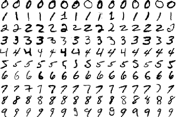
Image Provided by the MNIST handwritten database
You could imagine trying to devise a set of rules to distinguish each individual digit. Zeros, for instance, are basically one closed loop. But what if the person didn't perfectly close the loop. Or what if the right top of the loop closes below where the left top of the loop starts?
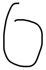
A zero that's difficult to distinguish from a six algorithmically
In this case, we have difficulty differentiating zeroes from sixes. We could establish some sort of cutoff, but how would you decide the cutoff in the first place? As you can see, it quickly becomes quite complicated to compile a list of heuristics (i.e., rules and guesses) that accurately classifies handwritten digits.
And there are so many more classes of problems that fall into this category. Recognizing objects, understanding concepts, comprehending speech. We don't know what program to write because we still don't know how it's done by our own brains. And even if we did have a good idea about how to do it, the program might be horrendously complicated.
So instead of trying to write a program, we try to develop an algorithm that a computer can use to look at hundreds or thousands of examples (and the correct answers), and then the computer uses that experience to solve the same problem in new situations. Essentially, our goal is to teach the computer to solve by example, very similar to how we might teach a young child to distinguish a cat from a dog.
Over the past few decades, computer scientists have developed a number of algorithms that try to allow computers to learn to solve problems through examples. Deep learning, which was first theorized in the early 80's (and perhaps even earlier), is one paradigm for performing machine learning. And because of a flurry of modern research, deep learning is again on the rise because it's been shown to be quite good at teaching computers to do what our brains can do naturally.
One of the big challenges with traditional machine learning models is a process called feature extraction. Specifically, the programmer needs to tell the computer what kinds of things it should be looking for that will be informative in making a decision. Feeding the algorithm raw data rarely ever works, so feature extraction is a critical part of the traditional machine learning workflow. This places a huge burden on the programmer, and the algorithm's effectiveness relies heavily on how insightful the programmer is. For complex problems such as object recognition or handwriting recognition, this is a huge challenge.
Deep learning is one of the only methods by which we can circumvent the challenges of feature extraction. This is because deep learning models are capable of learning to focus on the right features by themselves, requiring little guidance from the programmer. This makes deep learning an extremely powerful tool for modern machine learning.
A First Look at Neural Networks
Deep learning is a form of machine learning that uses a model of computing that's very much inspired by the structure of the brain. Hence we call this model a neural network. The basic foundational unit of a neural network is the neuron, which is actually conceptually quite simple.
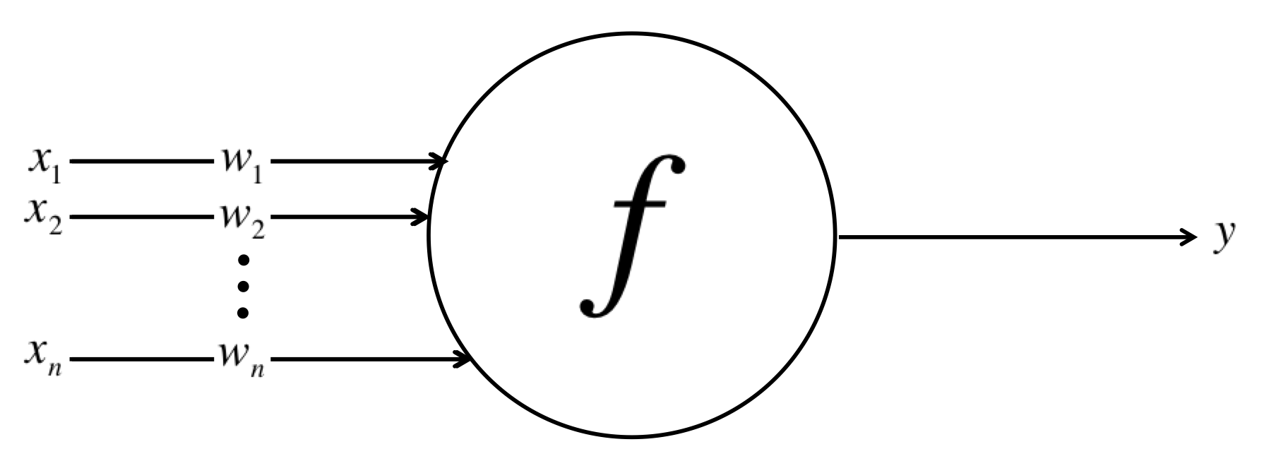
Schematic for a neuron in a neural net
Each neuron has a set of inputs, each of which is given a specific weight. The neuron computes some function on these weighted inputs. A linear neuron takes a linear combination of the weighted inputs. A sigmoidal neuron does something a little more complicated:
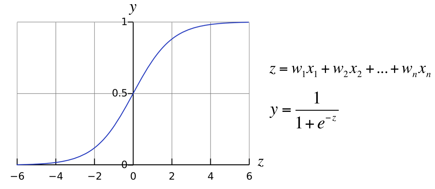
The function of a sigmoidal neuron
It feeds the weighted sum of the inputs into the logistic function. The logistic function returns a value between 0 and 1. When the weighted sum is very negative, the return value is very close to 0. When the weighted sum is very large and positive, the return value is very close to 1. For the more mathematically inclined, the logistic function is a good choice because it has a nice looking derivative, which makes learning a simpler process. But technical details aside, whatever function the neuron uses, the value it computes is transmitted to other neurons as its output. In practice, sigmoidal neurons are used much more often than linear neurons because they enable much more versatile learning algorithms compared to linear neurons.
A neural network comes about when we start hooking up neurons to each other, to the input data, and to the "outlets," which correspond to the network's answer to the learning problem. To make this structure easier to visualize, I've included a simple example of a neural net below. We let be the weight of the link connecting the neuron in the layer with the neuron in the layer:
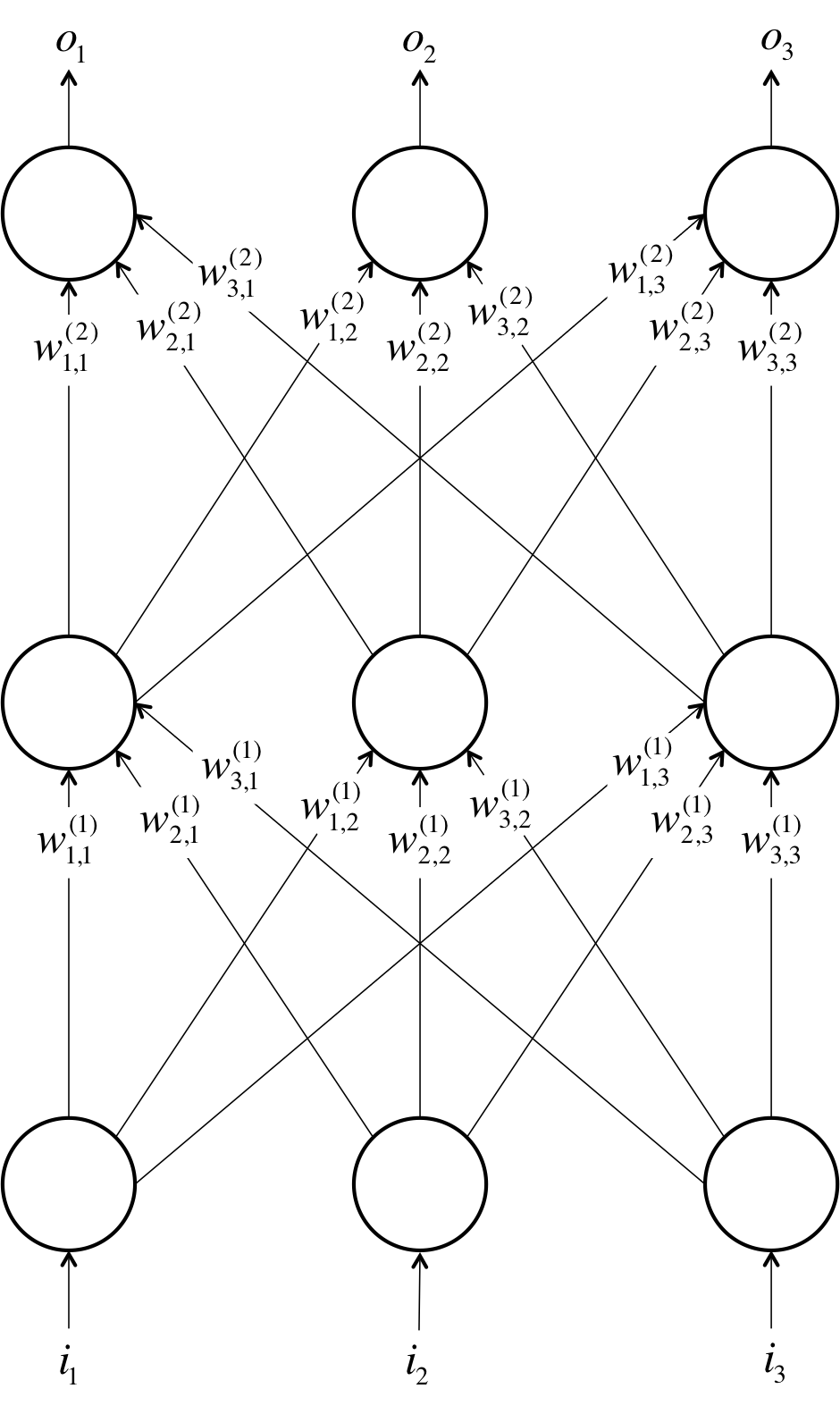
An example of a neural net with 3 layers and 3 neurons per layer
Similar to how neurons are generally organized in layers in the human brain, neurons in neural nets are often organized in layers as well, where neurons on the bottom layer receive signals from the inputs, where neurons in the top layers have their outlets connected to the "answer," and where are usually no connections between neurons in the same layer (although this is an optional restriction, more complex connectivities require more involved mathematical analysis). We also note that in this example, there are no connections that lead from a neuron in a higher layer to a neuron in a lower layer (i.e., no directed cycles). These neural networks are called feed-forward neural networks as opposed to their counterparts, which are called recursive neural networks (again these are much more complicated to analyze and train). For the sake of simplicity, we focus only on feed-forward networks throughout this discussion. Here's a set of some more important notes to keep in mind:
1) Although every layer has the same number of neurons in this example, this is not necessary.
2) It is not required that a neuron has its outlet connected to the inputs of every neuron in the next layer. In fact, selecting which neurons to connect to which other neurons in the next layer is an art that comes from experience. Allowing maximal connectivity will more often than not result in overfitting, a concept which we will discusss in more depth later.
3) The inputs and outputs are vectorized representations. For example, you might imagine a neural network where the inputs are the individual pixel RGB values in an image represented as a vector. The last layer might have 2 neurons which correspond to the answer to our problem: if the image contains a dog, if the image contains a cat, if it contains neither, and if it contains both.
4) The layers of neurons that lie sandwiched between the first layer of neurons (input layer) and the last layer of neurons (output layer), are called hidden layers. This is because this is where most of the magic is happening when the neural net tries to solve problems. Taking a look at the activities of hidden layers can tell you a lot about the features the network has learned to extract from the data.
Training a Single Neuron
Well okay, things are starting to get interesting, but we're still missing a big chunk of the picture. We know how a neural net can compute answers from inputs, but we've been assuming that we know what weights to use to begin with. Finding out what those weights should be is the hard part of the problem, and that's done through a process called training. During training, we show the neural net a large number of training examples and iteratively modify the weights to minimize the errors we make on the training examples.
Let's start off with a toy example involving a single linear neuron to motivate the process. Every day you grab lunch in the dining hall where your meal consists completely of burgers, fries, and soda. You buy some number of servings of each item. You want to be able to predict how much your meal will cost you, but you don't know the prices of each individual item. The only thing the cashier will tell you is the total price of the meal.
How do we solve this problem? Well, we could begin by being smart about picking our training cases, right? For one meal we could buy only a single serving of burgers, for another we could only buy a single serving of fries, and then for our last meal we could buy a single serving of soda. In general, choosing smart training cases is a very good idea. There's lots of research that shows that by engineering a clever training set, you can make your neural net a lot more effective. The issue with this approach is that in real situations, this rarely ever gets you even 10% of the way to the solution. For example, what's the analog of this strategy in image recognition?
Let's try to motivate a solution that works in general. Take a look at the single neuron we want to train:

The neuron we want to train for the Dining Hall Problem
Let's say we have a bunch of training examples. Then we can calculate what the neural network will output on the training example using the simple formula in the diagram. We want to train the neuron so that we pick the optimal weights possible - the weights that minimize the errors we make on the training examples. In this case, let's say we want to minimize the square error over all of the training examples that we encounter. More formally, if we know that is the true answer for the training example and is the value computed by the neural network, we want to minimize the value of the error function :
Now at this point you might be thinking, wait up... Why do we need to bother ourselves with this error function nonsense when we have a bunch of variables (weights) and we have a set of equations (one for each training example)? Couldn't we just solve this problem by setting up a system of linear system of equations? That would automaically give us an error of zero assuming that we have a consistent set of training examples, right?
That's a smart observation, but the insight unfortunately doesn't generalize well. Remember that although we're using a linear neuron here, linear neurons aren't used very much in practice because they're constrained in what they can learn. And the moment you start using nonlinear neurons like the sigmoidal neurons we talked about, we can no longer set up a system of linear equations!
So maybe we can use an iterative approach instead that generalizes to nonlinear examples. Let's try to visualize how we might minimize the squared error over all of the training examples by simplifying the problem. Let's say we're dealing with a linear neuron with only two inputs (and thus only two weights, and ). Then we can imagine a 3-dimensional space where the horizontal dimensions correspond to the weights and , and there is one vertical dimension that corresponds to the value of the error function . So in this space, points in the horizontal plane correspond to different settings of the weights, and the height at those points corresponds to the error that we're incurring, summed over all training cases. If we consider the errors we make over all possible weights, we get a surface in this 3-dimensional space, in particular a quadratic bowl:
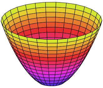
The quadratic error surface for a linear neuron
We can also conveniently visualize this surface as a set of elliptical contours, where the minimum error is at the center of the ellipses:
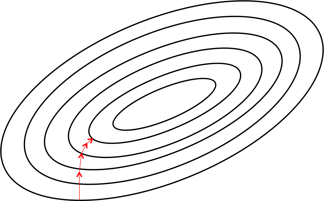
Visualizing the error surface as a set of contours
So now let's say we find ourselves somewhere on the horizontal plane (by picking a random initialization for the weights). How would we get ourselves to the point on the horizontal plane with the smallest error value? One strategy is to always move perpendicularly to the contour lines. Take a look, for instance, at the path denoted by the red arrows. Quite clearly, you can see that following this strategy will eventually get us to the point of minimum error.
What's particularly interesting is that moving perpendicularly to the contour lines is equivalent to taking the path of steepest descent down the parabolic bowl. This is a pretty amazing result from calculus, and it gives us the name of this general strategy for training neural nets: gradient descent.
Learning Rates and the Delta Rule
In practice at each step of moving perpendicular to the contour, we need to determine how far we want to walk before recalculating our new direction. This distance needs to depend on the steepness of the surface. Why? The closer we are to the minimum, the shorter we want to step forward. We know we are close to the minimum, because the surface is a lot flatter, so we can use the steepness as an indicator of how close we are to the minimum. We multiply this measure of steepness with a pre-determined constant factor , the learning rate. Picking the learning rate is a hard problem. If we pick a learning rate that's too small, we risk taking too long during the training process. If we pick a learning rate that's too big, we'll mostly likely start diverging away from the minimum (this pretty easy to visualize). Modern training algorithms adapt the learning rate to overcome this difficult challenge.
For those who are interested, putting all the pieces results in what is called the delta rule for training the linear neuron. The delta rule states that given a learning rate , we ought to change the weight at each iteration of training by . Deriving this formula is left as an exercise for the experienced reader. For a hint, study our derivation for a sigmoidal neuron in the next section.
Unfortunately, just taking the path of steepest descent doesn't always do the trick when we have nonlinear neurons. The error surface can get complicated and there could be multiple local minimum. As a result, using this procedure could potentially get us to a bad local minimum that isn't the global minimum. As a result, in practice, training neural nets involves a modification of gradient descent called stochastic gradient descent, that tries to use randomization and noise to find the global minimum with high probability on a complex error surface.
Moving onto the Sigmoidal Neuron *
This section and the next will get a little heavy with the math, so just be forewarned. If you're not comfortable with multivariate calculus, feel free to skip them and move onto the remaining sections. Otherwise, let's just dive right into it!
Let's recall the mechanism by which logistic neurons compute their output value from their inputs:
The neuron computes the weighted sum of its inputs, the logit, . It then feeds into the input function to compute , its final output. These functions have very nice derivatives, which makes learning easy! For learning, we want to compute the gradient of the error function with respect to the weights. To do so, we start by taking the derivative of the logit, , with respect to the inputs and the weights. By linearity of the logit:
Also, quite surprisingly, the derivative of the output with respect to the logit is quite simple if you express it in terms of the output. Verifying this is left as an exercise for the reader:
We then use the chain rule to get the derivative of the output with respect to each weight:
Putting all of this together, we can now compute the derivative of the error function with respect to each weight:
Thus, the final rule for modifying the weights becomes:
As you may notice, the new modification rule is just like the delta rule, except with extra multiplicative terms included to account for the logistic component of the sigmoidal neuron.
The Backpropagation Algorithm *
Now we're finally ready to tackle the problem of training multilayer neural networks (instead of just single neurons). So what's the idea behind backpropagation? We don't know what the hidden units ought to be doing, but what we can do is compute how fast the error changes as we change a hidden activity. Essentially we'll be trying to find the path of steepest descent!
Each hidden unit can affect many output units. Thus, we'll have to combine many separate effects on the error in an informative way. Our strategy will be one of dynamic programming. Once we have the error derivatives for one layer of hidden units, we'll use them to compute the error derivatives for the activites of the layer below. And once we find the error derivatives for the activities of the hidden units, it's quite easy to get the error derivatives for the weights leading into a hidden unit. We'll redefine some notation for ease of discussion and refer to the following diagram:

Reference diagram for the derivation of the backpropagation algorithm
The subscript we use will refer to the layer of the neuron. The symbol will refer to the activity of a neuron, as usual. Similarly the symbol will refer to the logit of a neuron. We start by taking a look at the base case of the dynamic programming problem, the error function derivatives at the output layer:
Now we tackle the inductive step. Let's presume we have the error derivatives for layer . We now aim to calculate the error derivatives for the layer below it, layer . To do so, we must accumulate information for how the output of a neuron in layer affects the logits of every neuron in layer . This can be done as follows, using the fact that the partial derivative of the logit with respect to the incoming output data from the layer beneath is merely the weight of the connection :
Now we can use the following to complete the inductive step:
Combining these two together, we can finally express the partial derivatives of layer in terms of the partial derivatives of layer .
Then once we've gone through the whole dynamic programming routine, having filled up the table appropriately with all of our partial derivatives (of the error function with respect to the hidden unit activities), we can then determine how the error changes with respect to the weights. This gives us how to modify the weights after each training example:
In order to do backpropagation with batching of training examples, we merely sum up the partial derivatives over all the training examples in the batch. This gives us the following modification formula:
We have succeeded in deriving the backpropagation algorithm for a feed-forward neural net utilizing sigmoidal neurons!
The Problem of Overfitting
Now let's say you decide you're very excited about deep learning and so you want to try to train a neural network of your own to identify objects in an image. You know this is a complicated problem so you use a huge neural network (let's say 20 layers) and you have 1,000 training examples. You train your neural network using the algorithm we describe, but something's clearly wrong. Your neural net performs virtually perfectly on your training examples, but when you put it in practice, it performs very poorly! What's going on here?
The problem we've encountered is called overfitting, and it happens when you have way too many parameters in your model and not enough training data. To visualize this, let's consider the figure below, where you want to fit a model to the data points:
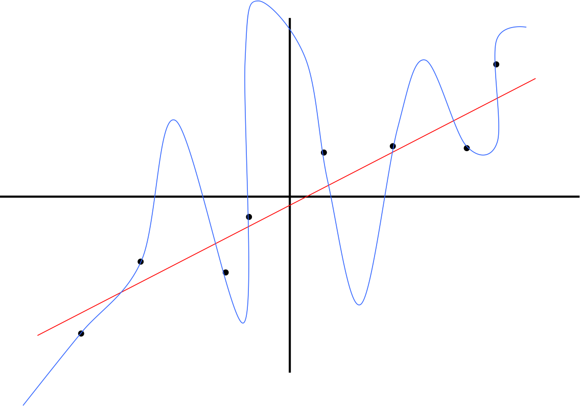
An example that illustrates the concept of overfitting
Which curve would you trust? The line which gets almost no training example exactly? Or the complicated curve that hits every single point in the training set? Most likely you would trust the linear fit instead of the complicated curve because it seems less contrived. This situation is analagous to the neural network we trained. We have way too many parameters, over 100 trillion trillion (or 100 septillion) parameters. It's no wonder that we're overfitting!
So how do we prevent overfitting? The two simplest ways are:
1) Limit the connectivities of neurons in your model. Architecting a good neural network requires a lot of experience and intuition, and it boils down to giving your model freedom to discover relationships while also constraining it so it doesn't overfit.
2) Adding more training examples! Often times you can cleverly add amplify your existing training set (changing illumination, applying shifts and other transformations, etc.).
There are more sophisticated methods of training that try to directly solve overfitting such as including a dropout layers/neurons, but these methods are beyond the scope of this article
Conclusions
We've covered a lot of ground, but there's still a lot more that's going on in deep learning research. In future articles, I will probably talk more about different kinds of neural architectures (convolutional networks, soft max layers, etc.). I'll probably also write an article about how to train your own neural network using some of the awesome open source libraries out there, such as Caffe (which allows you to GPU accelerate the training of neural networks). Those of you who are interested in pursuing deep learning further, please get in touch! I love talking about new ideas and projects ❤
