A Deep Dive into Recurrent Neural Nets
11 January 2015Last time, we talked about the traditional feed-forward neural net and concepts that form the basis of deep learning. These ideas are extremely powerful! We saw how feed-forward convolutional neural networks have set records on many difficult tasks including handwritten digit recognition and object classification. And even today, feed-forward neural networks consistently outperform virtually all other approaches to solving classification tasks.
And yet, despite their well celebrated successes, most experts would agree that feed-forward neural nets are still rather limited in what they can achieve. Why? Because the task of "classification" is only one small component of the incredible computational power of the human brain. We're wired not only to recognize individual instances but to also analyze entire sequences of inputs. These sequences are ultra rich in information, have complex time dependencies, and can be of arbitrary length. For example, vision, motor control, speech, and comprehension all require us to process high-dimensional inputs as they change over time. This is something that feed-forward nets are incredibly poor at modeling.
What is a Recurrent Neural Net?
One quite promising solution to tackling the problem of learning sequences of information is the recurrent neural network (RNN). RNNs are built on the same computational unit as the feed forward neural net, but differ in the architecture of how these neurons are connected to one another. Feed forward neural networks were organized in layers, where information flowed unidirectionally from input units to output units. There were no undirected cycles in the connectivity patterns. Although neurons in the brain do contain undirected cycles as well as connections within layers, we chose to impose these restrictions to simplify the training process at the expense of computational versatility. Thus, to create more powerful compuational systems, we allow RNNs to break these artificially imposed rules. RNNs do not have to be organized in layers and directed cycles are allowed. In fact, neurons are actually allowed to be connected to themselves.

An example schematic of a RNN with directed cycles and self connectivities
The RNN consists of a bunch of input units, labeled and output units, labeled . There are also the hidden units , which do most of the interesting work. You'll notice that the illustration shows a unidirectional flow of information from the input units to the hidden units as well as another unidirectional flow of information from the hidden units to the output units. In some cases, RNNs break the latter restriction with connections leading from the output units back to the hidden units. These are called "backprojections," and don't make the analysis of RNNs too much more complicated. The same techniques we will discuss here will also apply to RNNs with backprojections.
There are a lot of pretty challenging technical difficulties that arise when training recurrent neural networks, and it's still a very active area of research. Hopefully by the end of this article, we'll have a solid understanding of how RNNs work and some of the results that have been achieved!
Simulating a Recurrent Neural Network
Now that we understand how a RNN is structured, we can discuss how it's able to simulate a sequence of events. Let's consider a neat toy example of a recurrent neural net acting like an timer module, a classic example designed by Herbert Jaeger (his original manuscript can be found here).

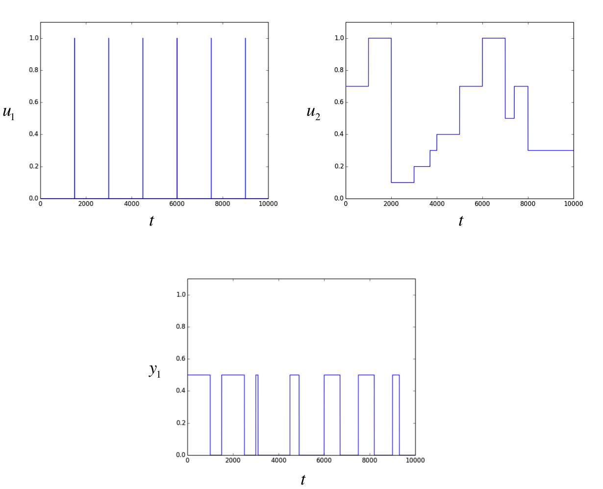
A simple example of how a perfect RNN would simulate a timer
In this case, we have two inputs. The input corresponds to a binary switch which spikes to one when the RNN is supposed to start the timer. The input is a discrete variable that varies between 0.1 and 1.0 inclusive which corresponds to how long the output should be turned on if the timer is started at that instant. The RNN's specification requires it to turn on the output for a duration of . Finally, the outputs in the training examples toggle between 0 (off) and 0.5 (on).
But how exactly would a neural net achieve this calculation? First, the RNN has all of its hidden activities initialized to some pre-determined state. Then at each time step (time ), every hidden unit sends its current activity through all its outgoing connections. It then recalculate its new activity by computing the weighted sum (logit) of its inputs from other neurons (including itself if there is a self connection) and the current values of the inputs, and then feeding this value into a neuron-specific function (a straightforward copy operation, sigmoid transform, soft-max, etc.). Because the previous vector of activities is used to compute the vector of activies in each time step, RNNs are able to retain memory of previous events and utlize this memory in making decisions.
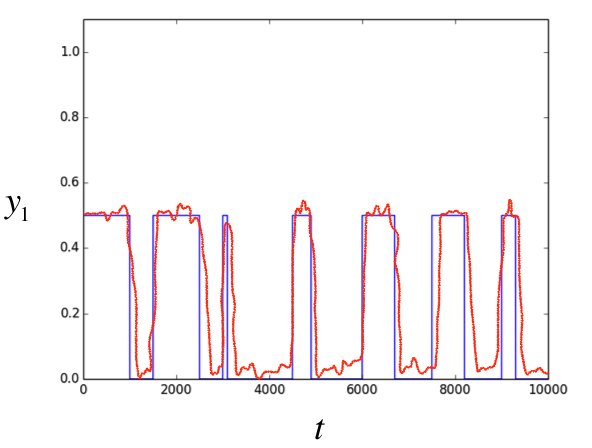
Clearly a neural net would be unlikely to perfectly perform according to specification, but you can imagine it outputting a result (orange) that looks pretty darn close to the ground truth (blue) after training the RNN with hundreds or thousands of examples. We'll talk more about approaches to training RNNs in the following sections.

An example fit for how a well-trained RNN might approximate the output of a test case
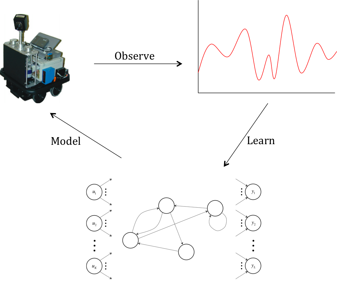
At this point, you're probably thinking that this is pretty cool, but it's still a pretty contrived example. What's the strategy for using RNNs in practice? We examine real systems and their behaviors over time in response to stimuli. For example, you might teach a RNN to transcribe audio into text by building a dataset (in a sense, observing the response of the human auditory system in response to the inputs in the training set). You may also use a trained neural net to model a system's reactions under novel stimuli.

How a RNN might be used in practice
But if you're creative, you can use RNNs in ways that seem pretty spectacular. For example, a specialized kind of RNN, called a long short-term RNN or LSTM, has been used to achieve spectacular rates of data compression (although the current approach to RNN-based compression does take a significant amount time). For those itching to learn more, we'll talk about the LSTM architecture in a later section.
Training a RNN - Backpropagation Through Time
Great, now we understand what a RNN is and how it works, but how do we train a RNN in the first place to achieve all of these spectacular feats? Specifically, how do we determine the weights that are on each of the connections? And how do we choose the initial activities of all of the hidden units? Our first instinct might be to use backpropagation directly, after all it worked quite well when we used it on feed forward neural nets.
The problem with using backpropagation here is that we have cyclical dependencies. In feed forward nets, when we calculated the error derivatives with respect to the weights in one layer, we could express them completely in terms of the error derivatives from the layer above. In a recurrent neural network, we don't have this nice layering because the neurons do not form a directed acyclic graph. Trying to backpropagate through a RNN could force us to try to express an error derivative in terms of itself, which doesn't make for easy analysis.
So how can we use backpropagation for RNNs, if at all? The answer lies in employing a clever transformation, where we convert our RNN into a new structure that's essentially a feed-forward neural network! We call this strategy "unrolling" the RNN through time, and an example can be seen in the figure below (with only one input/output per time step to simplify the illustration):

An example of "unrolling" and RNN through time to use backpropagation
The process is actually quite simple, but it has a profound impact on our ability to analyze the neural network. We take the RNN's inputs, outputs, and hidden units and replicate it for every time step. These replications correspond to layers in our new feed forward neural network. We then connect hidden units as follows. If the original RNN has a connection of weight from neuron to neuron , in our feed forward neural net, we draw a connection of weight from neuron in every layer to neuron in every layer .
Thus, to train our RNN, we randomly initialize the weights, "unroll" it into a feed forward neural net, and backpropogate to determine the optimal weights! To determine the initializations for the hidden states at time 0, we can treat the initial activities as parameters fed into the feed forward network at the lowest layer and backpropagate to determine their optimal values as well!
We run into a problem however, which is that after every batch of training examples we use, we need to modify the weights based on the error derivatives we calculated. In our feed-forward net, we have sets of connections that all correspond to the same connection in the original RNN. The error derivatives calculated with respect to their weights, however, are not guaranteed to be equal, which means we might be modifying them by different amounts. We definitely don't want to be doing that!
We can get around this challenge, by averaging (or summing) the error derivatives over all the connections that belong to the same set. This means that after each batch, we modify corresponding connections by the same amount, so if they were initialized to the same value, they will end up at the same value. This solves our problem :)
The Problems with Deep Backpropagation
Unlike traditional feed forward nets, the feed forward nets generated by unrolling RNNs can be enormously deep. This gives rise to a serious practical issue: it can be obscenely difficult to train using the backpropagation through time approach. Let's take a step back and try to understand why.
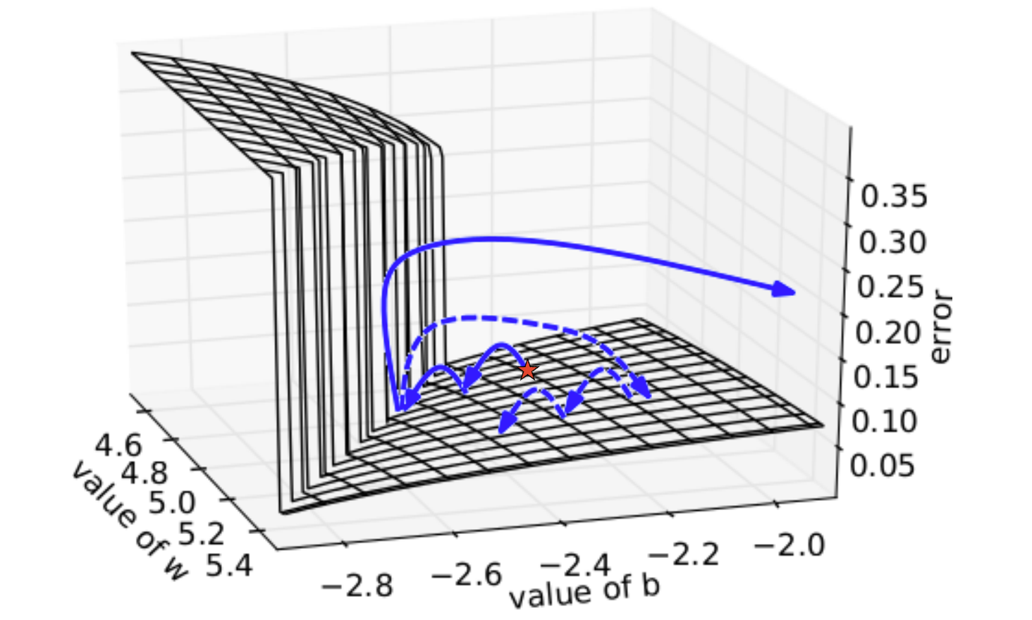
Let's try to train a RNN to do a very primitive task. Let's give the RNN a single hidden unit with a bias term, and we'll connect it to itself and a singular output. We want this neural network to output a fixed target value after 50 steps, let's say 0.7. We'll use the squared error of the output on the 50th time step as our error function, which we can plot as a surface over the value of the weight and the bias:

The problematic error surface of a simple RNN (image from: Pascanu et al.)
Now, let's say we started at the red star (using a random initialization of weights). You'll notice that as we use gradient descent, we get closer and closer to the local minimum on the surface. But suddenly, when we slightly overreach the valley and hit the cliff, we are presented with a massive gradient in the opposite direction. This forces us to bounce extremely far away from the local minimum. And once we're in nowhere land, we quickly find that the gradients are so vanishingly small that coming close again will take a seemingly endless amount of time. This issue is called the problem of exploding and vanishing gradients. You can imagine perhaps controlling this issue by rescaling gradients to never exceed a maximal magnitude (see the dotted path after hitting the cliff), but this approach still doesn't perform spectacularly well, especially in more complex RNNs. For a more mathematical treatment of this issue, check out this paper.
Long Short Term Memory
To address these problems, researchers proposed a modified architecture for recurrent neural networks to help bridge long time lags between forcing inputs and appropriate responses and protect against exploding gradients. The architecture forces constant error flow (thus, neither exploding nor vanishing) through the internal state of special memory units. This long short term memory (LSTM) architecture utlized units that were structured as follows:

Structure of the basic LSTM unit
The LSTM unit consists of a memory cell which attempts to store information for extended periods of time. Access to this memory cell is protected by specialized gate neurons - the keep, write, and read gates - which are all logistic units. These gate cells, instead of sending their activities as inputs to other neurons, set the weights on edges connecting the rest of the neural net to the memory cell. The memory cell is a linear neuron that has a connection to itself. When the keep gate is turned on (with an activity of 1), the self connection has weight one and the memory cell writes its contents into itself. When the keep gate outputs a zero, the memory cell forgets its previous contents. The write gate allows the rest of the neural net to write into the memory cell when it outputs a 1 while the read gate allows the rest of the neural net to read from the memory cell when it outputs a 1.
So how exactly does this force a constant error flow through time to locally protect against exploding and vanishing gradients? To visualize this, let's unroll the LSTM unit through time:

Unrolling the LSTM unit through the time domain
At first, the keep gate is set to 0 and the write gate is set to 1, which places 4.2 into the memory cell. This value is retained in the memory cell by a subsequent keep value of 1 and protected from read/write by values of 0. Finally, the cell is read and then cleared. Now we try to follow the backpropagation from the point of loading 4.2 into the memory cell to the point of reading 4.2 from the cell and its subsequent clearing. We realize that due to the linear nature of the memory neuron, the error derivative that we receive from the read point backpropagates with negligible change until the write point because the weights of the connections connecting the memory cell through all the time layers have weights approximately equal to 1 (approximate because of the logistic output of the keep gate). As a result, we can locally preserve the error derivatives over hundreds of steps without having to worry about exploding or vanishing gradients. You can see the action of this method successfully reading cursive handwriting:
The animation, borrowed from neural networks expert Alex Graves, requires a little bit of explanation:
1) Row 1: Shows when the letters are recognized
2) Row 2: Shows the states of some of the memory cells (Notice how they get reset when a character is recognized!)
3) Row 3: Shows the writing as it's being analyzed by the LSTM RNN
4) Row 4: This shows the gradient backpropagated to the inputs from the most active character of the upper soft-max layer (This tells you which data points are providing the most influence on your current decision for the character)
The LSTM RNN does quite well, and it's been applied in lots of other places as well. As we discussed earlier, deep architectures for LSTM RNNs have been used to achieve pretty astonishing data compression rates. For those who are interested in learning more about this particular application for LSTM RNNs can check out this paper.
Conclusions
How to effectively train neural nets remains an area of active research and has resulted in a number of alternative approaches, with no clear winner. The LSTM RNN architecture is one such approach to improving the training of RNNs. Another approach is to use a much better optimzer that can deal with exploding and vanishing gradients. Hessian-free optimization tries to detect directions with a small gradient, but even smaller curvature. This problem allows it to perform much better than naive gradient descent. A third approach involves a very careful initialization of the weights in hopes that it will allow us to avoid the problem of exploding and vanishing gradients in the first place (e.g. echo state networks, momentum based approaches).
RNNs are pretty powerful stuff, and I'm quite excited to see what comes out of this area of active research over the next few years. If any of these topics that I briefly touched upon in the previous paragraph seem interesting, shoot me an email at [email protected]! I can write another blog post exploring other approaches to RNNs. Thanks for all of the support and I hope you enjoy this article ❤
